Understanding how FCAs impact battery operations and dispatch optimization in Germany
Flexible Connection Agreements (FCAs) impose operational constraints on grid-connected assets. As grid capacity becomes increasingly constrained, FCAs are emerging as a mechanism for enabling new connections while managing network limitations.
Read this article to learn more about how FCAs impact revenues and why the dispatch varies as shown below.
Ramping Rate Restrictions
FCA agreements may limit how quickly a battery can change its power output. The model enforces four directional ramp constraints:
Ramp-up limits (increasing power):
\[P^{\text{charge}}_t - P^{\text{charge}}_{t-1} \leq R^{\max}_{\Delta t}\] \[P^{\text{discharge}}_t - P^{\text{discharge}}_{t-1} \leq R^{\max}_{\Delta t}\]Ramp-down limits (decreasing power):
\[P^{\text{charge}}_t - P^{\text{charge}}_{t-1} \geq -R^{\max}_{\Delta t}\] \[P^{\text{discharge}}_t - P^{\text{discharge}}_{t-1} \geq -R^{\max}_{\Delta t}\]Where \(R^{\max}_{\Delta t}\) is the maximum allowed power change per timestep.
Average Power During Ramping
When ramp times are non-zero, the battery cannot instantly reach its target power level. The model calculates average power during each period using the trapezoidal rule to account for gradual ramping:
Power
(MW)
  │
  │  P_t^signal  ·······•─────────────────•
  │                    ╱                  │
  │                   ╱                   │
  │                  ╱                    │
  │                 ╱                     │
  │                ╱                      │
  │ P_{t-1}^signal •                       │
  │                │                      │
  └────────────────┼──────────────────────┼────► Time
                 t-1         τ            t
                   │←────────→│
                   │←────────────────────→│
                              Δt
Energy Calculation via Trapezoid Area:
The energy delivered during the timestep equals the area under the power curve. This area comprises two regions:
-
Ramp region (from \(t-1\) to \(t-1+\tau\)): A trapezoid with parallel sides \(P_{t-1}^{\text{signal}}\) and \(P_t^{\text{signal}}\)
-
Flat region (from \(t-1+\tau\) to \(t\)): A rectangle at \(P_t^{\text{signal}}\)
Using the trapezoid area formula \(A = \frac{1}{2}(a + b) \cdot h\):
\[E_t = \underbrace{\frac{1}{2}\left(P_{t-1}^{\text{signal}} + P_t^{\text{signal}}\right) \cdot \tau}_{\text{ramp region}} + \underbrace{P_t^{\text{signal}} \cdot (\Delta t - \tau)}_{\text{flat region}}\]Expanding and simplifying:
\[E_t = P_t^{\text{signal}} \cdot \Delta t - \frac{\tau}{2} \left(P_t^{\text{signal}} - P_{t-1}^{\text{signal}}\right)\]The average power over the timestep is therefore:
\[P^{\text{avg}}_t = \frac{E_t}{\Delta t} = P_t^{\text{signal}} - \frac{\tau}{2 \Delta t} \left(P_t^{\text{signal}} - P_{t-1}^{\text{signal}}\right)\]Or equivalently:
\[P^{\text{avg}}_t = P_{t-1}^{\text{signal}} + \frac{2\Delta t - \tau}{2 \Delta t} \cdot \left( P_t^{\text{signal}} - P_{t-1}^{\text{signal}} \right)\]Boundary Cases:
| Ramp Time | Average Power | Interpretation |
|---|---|---|
| \(\tau = 0\) | \(P^{\text{avg}}_t = P_t^{\text{signal}}\) | Instantaneous ramping—power jumps immediately |
| \(\tau = \Delta t\) | \(P^{\text{avg}}_t = \frac{P_{t-1}^{\text{signal}} + P_t^{\text{signal}}}{2}\) | Full-period ramp—linear interpolation |
Instantaneous (τ = 0)          With Ramp Time (τ > 0)
─────────────────────          ─────────────────────
Power                          Power
  │       ┌────────              │            ┌──────
  │       │                      │           ╱│
  │       │                      │          ╱ │
  │       │                      │         ╱  │
  │───────┘                      │────────╱   │
  └──────────────► t             └──────────────► t
        t-1    t                       t-1  τ  t

  Area = P_t × Δt                Area = trapezoid + rectangle
  (full rectangle)               (accounts for gradual ramp)
Export/Import Limits
Flexible connections often impose time-varying limits on grid export or import:
\[P^{\text{export}}_t \leq P^{\text{FCA,export}}_t \quad \text{and} \quad P^{\text{import}}_t \leq P^{\text{FCA,import}}_t\]These constraints directly affect the battery’s ability to participate in wholesale markets and must be factored into dispatch decisions.
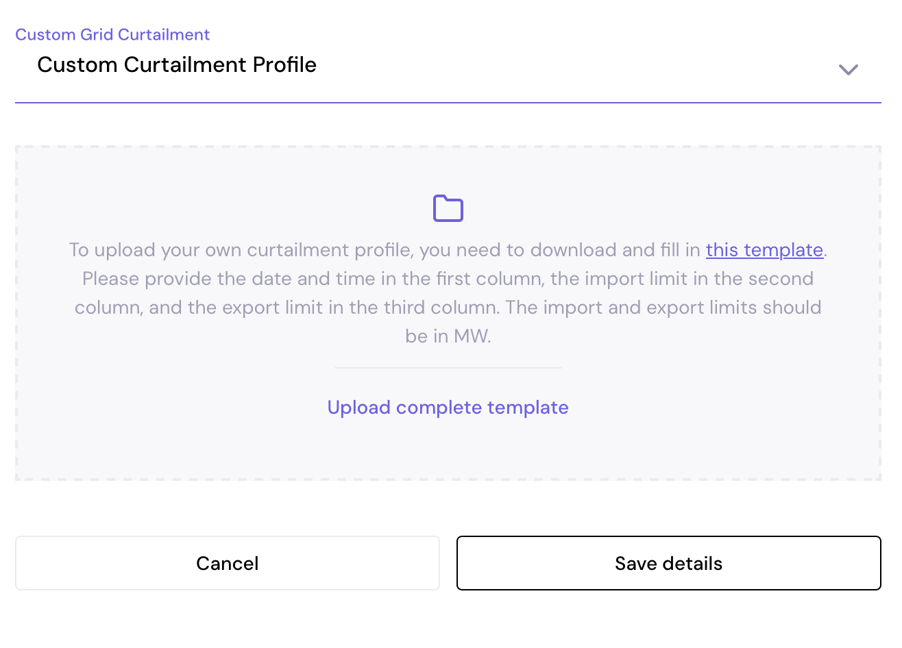
This is how custom curtailment profiles appear on the terminal:
Ancillary Service Participation
Under FCA, ancillary service participation may be restricted:
- Reduced FCR/aFRR capacity available due to export constraints
- Model adjusts maximum ancillary service provision based on FCA limits
- Revenue impact quantified by comparing constrained vs unconstrained dispatch
Related Pages
- Dispatch Model – How the model optimizes battery dispatch across German markets
- Revenue Stack – Overview of available revenue streams in Germany