Day-Ahead vs Intraday

How we build an intraday forecast

---

Our model produces an intraday (ID) price forecast as well as a day-ahead (DA) price forecast in each 15-minute time period.

Modelling intraday prices

The DA price of electricity is informed by forecasts for demand, wind and solar generation, and plant availability. These forecasts are critical to building the supply stack to meet demand from one settlement period to the next and setting power prices.

As time progresses from the closure of the day-ahead market to delivery, forecasts for each of these variables evolve towards the outturn values. The intraday markets allow power to be bought and sold in response to these changing forecasts until a specified time before the delivery window starts (time will depend on the intraday market).

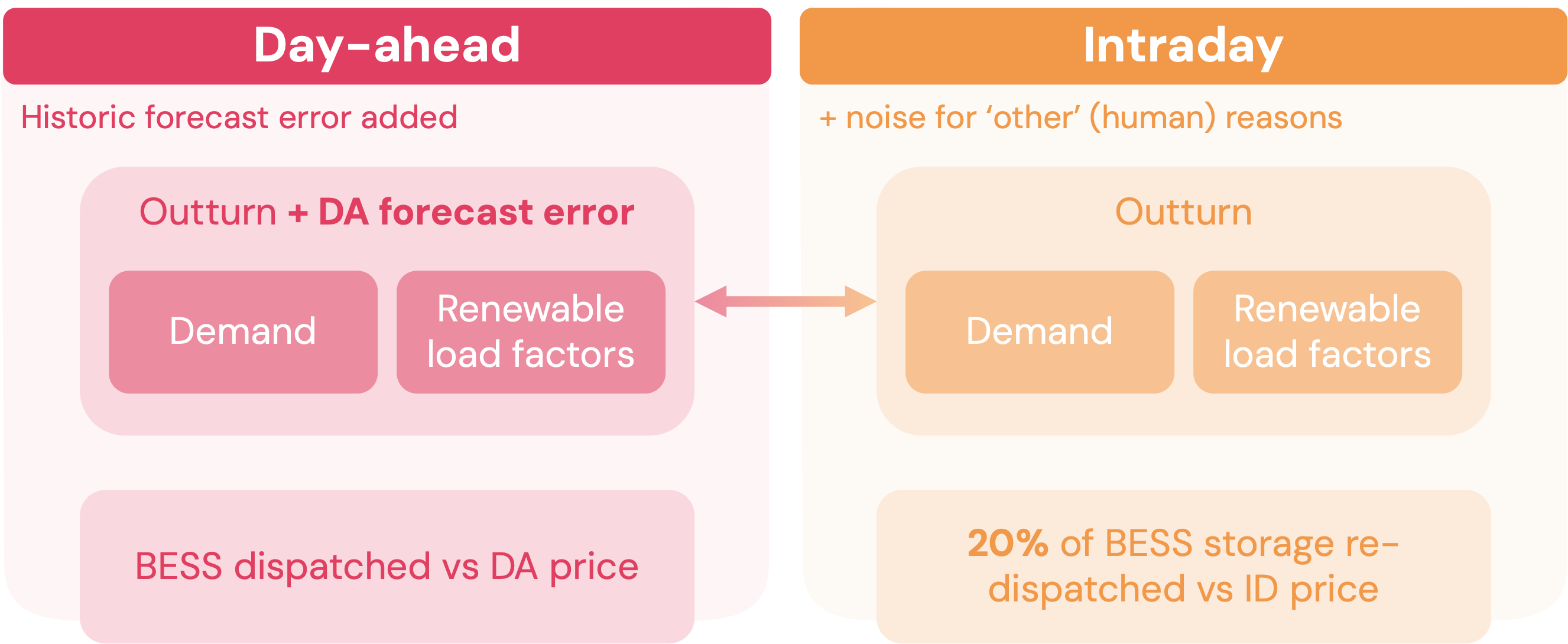
While the DA price and ID price are highly correlated, the evolution of these forecasts (along with human behaviours) causes intraday prices to diverge from their day-ahead reference point. These price changes represent an opportunity for storage to optimise against.

Learn more:

• Day-ahead forecast errors — How we model demand, wind, and solar generation forecast errors
• Other impacts to intraday pricing — How human behaviour affects intraday prices

Day-ahead forecast errors

Forecast errors lead to discrepancies between planned and actual behaviour of generation and storage assets

The difference between a forecast and what happens (the ‘outturn’) is the forecast error.

Forecast errors are modelled on historical data

We model day-ahead forecast errors on the following variables using historical data:

Variable	Error data source
Demand	NESO, ENTSO-E
Solar generation	NESO, ENTSO-E
Offshore wind generation	Elexon, ENTSO-E
Onshore wind generation	Elexon, ENTSO-E

Replicating observed patterns in forecast values of wind, solar and demand

Examining data from recent history, we find several trends.

Links between weather and likely error profiles

The wind forecast will likely be closer to the outturn value (i.e. the error is small) on particularly windy or non-windy days. It is those days that sit in the middle where the error is higher. It’s easier to say, ‘This will be a very windy day’ or ‘This will be a still day’ than ‘There will be a small amount of wind in the morning and a bit more in the afternoon’. The same thing applies to solar.

Within-day error correlations

In addition, if a forecast is lower than it should be at 8am, it will likely be low at 9am. A forecast will rarely bounce from higher than the outturn to lower than the outturn in each subsequent hour. There is a pattern to how a forecast’s error behaves across time called ‘autocorrelation’.

We want to preserve these properties when we project forward forecast errors between day-ahead and intraday markets. We do this by matching similar days in our historical ‘error year’ to those in our forecast weather year. To show how this works let’s look at solar in more detail.

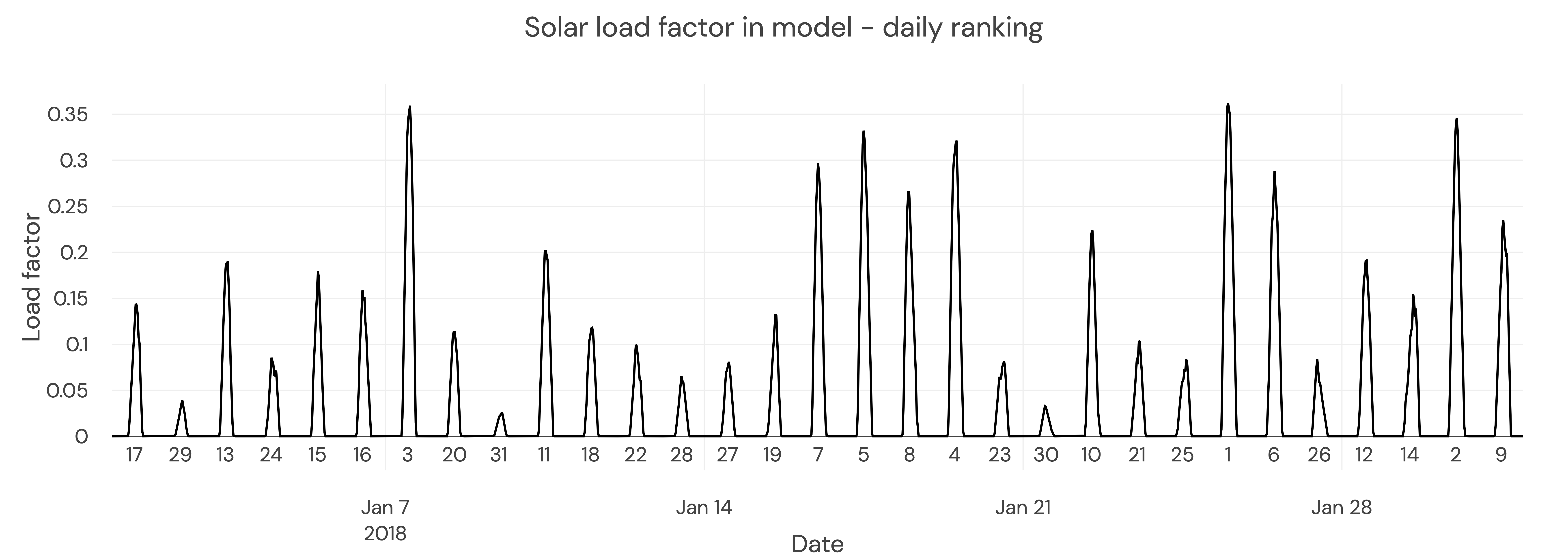
Matching similar days in an error-weather year to our forecast-weather year

For each month in the weather year, we rank days from highest to lowest load factor. This is 2018, the weather year we use in the forecast. This graph shows January in Great Britain: 25th was the sunniest day, so is labelled ‘1’.

We repeat the same process for the forecast error year 2019. In the graph below, ‘Day ahead’ is the solar production forecast a day before delivery, and ‘Intraday’ is the solar outturn value. We have ranked days from highest to lowest load factor using the intraday load factor as the reference.

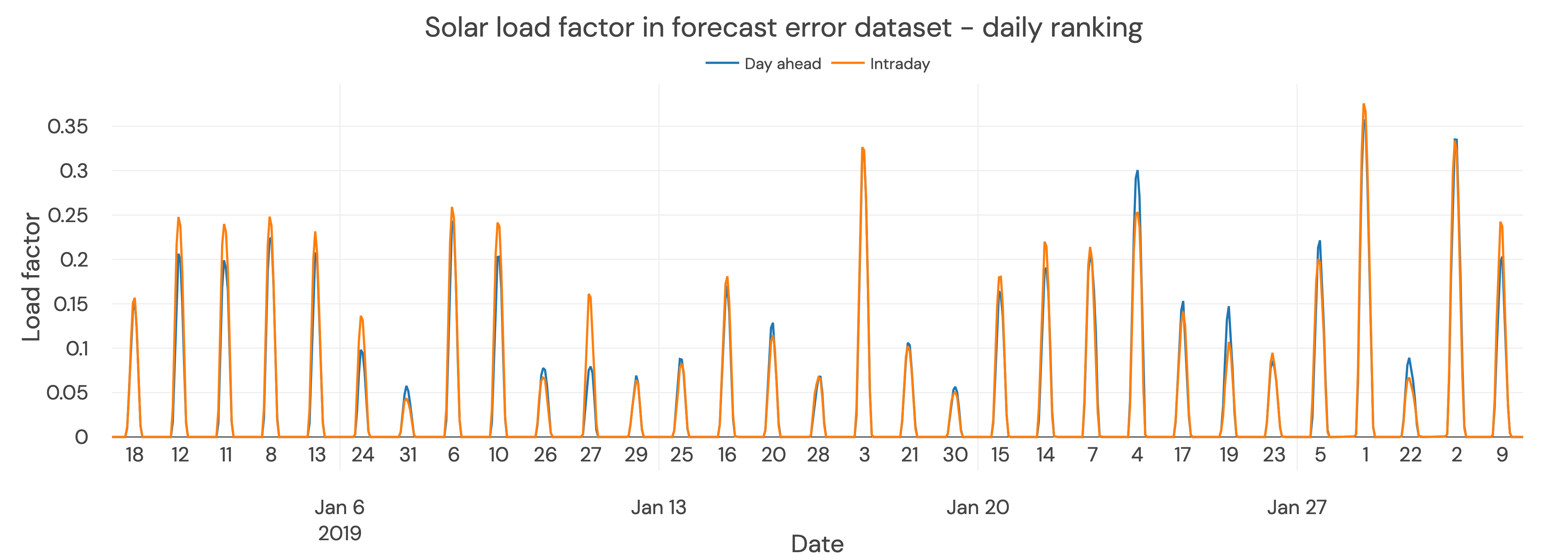
We match days in the weather year to days in the error year with the same rank. To estimate day-ahead load factors, we apply the percentage error in each settlement period from the error day to our intraday load factors. For example, the error from the sunniest day in January 2019 is applied to outturn data for the sunniest day in January 2018.

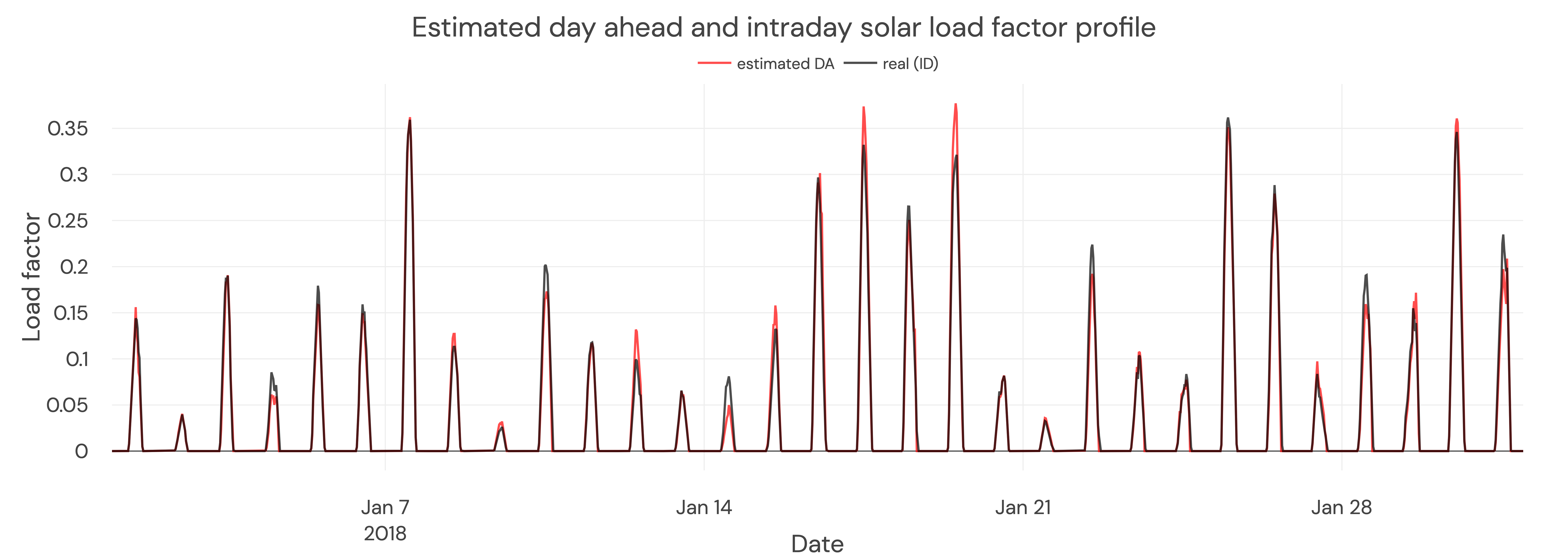
The load factor of the outturn production is used for the intraday price forecast. The load factor of the estimated day-ahead profile is used for the day-ahead price forecast. We apply the same principles to our demand and wind profiles to calculate the divergence between DA and ID prices based on forecast errors.

Other impacts to intraday pricing

There is more to the difference between day-ahead and intraday prices than just forecast errors: human behaviour also impacts prices in the intraday continuous market.

We make several assumptions in building the intraday price model that lead to an underestimation of volatility between DA and ID. We explain these assumptions and how we mitigate against them here.

Assumption 1: actual renewable generation and demand are known when ID prices are set

The intraday continuous market trades over the counter on a pay-as-bid basis. Each settlement period can be traded at thousands of different prices, at different times ranging from hours before delivery up until gate closure.

By using outturn forecasts for renewables and demand leads to a fundamentals intraday price that is closer to the intraday closing price than the volume-weighted average price of all intraday prices traded for each period. While most volume is traded in the last 90 minutes before delivery, we find that it is necessary to add additional noise to our intraday price forecast, to capture the additional uncertainty.

We base the magnitude of this noise on historical differences between volume-weighted average prices and intraday closing prices, modelling it using an AR(1) (first-order autoregressive) process to reflect the same autocorrelation observed in actual price deviations. This approach shifts our intraday price forecast from a closing price estimate to a more realistic volume-weighted price forecast.

AR(1) Noise Model

The AR(1) model generates time-correlated noise where each value depends on the previous value:

\[x_t = \rho \cdot x_{t-1} + \varepsilon_t\]

Where:

• \(\rho\) (persistence): The autocorrelation coefficient, controlling how strongly prices from one period influence the next
• \(\varepsilon_t\): White noise with variance \(\sigma_\varepsilon^2 = \sigma^2 \cdot (1 - \rho^2)\)
• \(\sigma\) (std_dev): The target standard deviation of the process

This structure ensures that if intraday prices deviate from day-ahead in one period, they are likely to continue deviating in the same direction in subsequent periods—matching observed market behaviour.

Kurtosis Adjustment

Historical intraday price deviations exhibit heavier tails than a normal distribution (i.e., extreme price spikes occur more frequently than a Gaussian model would predict). To capture this, we apply a power transform to the AR(1) noise:

\[\text{adjusted noise} = \text{sign}(x) \cdot |x|^p\]

Where \(p\) (kurtosis parameter) controls the heaviness of the distribution tails:

• \(p = 1.0\): No adjustment (standard normal tails)
• \(p > 1.0\): Heavier tails, more extreme values

After the transform, the noise is re-normalized to maintain the target standard deviation. The observed_std parameter allows us to calibrate against historical data.

Node-Specific Parameters

The noise model is configured per-node (e.g., Germany, Great Britain), allowing each market to have calibrated parameters based on its historical price behaviour.

Assumption 2: all trading behaviour is logical and rational

It is not just forecast uncertainty that can move intraday price - bidding behaviour also plays a significant role. In particular, “herding” is where traders or trading algorithms take decisions based more on the actions or signals of other participants than on their own analysis. This can cause amplification of price movements.

Other human behaviours, such as mistakes, can also cause fluctuations in prices. To capture this behaviour, we scale up the spread between day-ahead and intraday prices. For example, if the raw model calculates an intraday price 10 €/MWh higher than day-ahead, the final spread might be increased to 12 €/MWh.

When intraday prices are negative, scaling may be disabled to avoid amplifying negative spreads inappropriately.