Understanding how FCAs impact battery operations and dispatch optimization in Germany
Flexible Connection Agreements (FCAs) impose operational constraints on grid-connected assets. As grid capacity becomes increasingly constrained, FCAs are emerging as a mechanism for enabling new connections while managing network limitations.
Read this article to learn more about how FCAs impact revenues and why the dispatch varies as shown below.
Three settings control FCA restrictions in a forecast
Three FCA-related settings can be entered when creating a German forecast, all found in the forecast creation flow:
| Setting | Where | What it does |
|---|---|---|
| Ramp Time (Leistungsgradient) | Grid connection tab, in minutes | How long the battery would take to travel the full range from zero to rated power, up to 30 minutes. The model converts this into a ramp rate, so a smaller move takes proportionally less time than the figure entered. A longer ramp time reduces how quickly the battery can react to prices, and the forecast accounts for the energy lost while ramping. |
| Ancillary service limits | Grid connection tab, % of rated power ineligible for ancillary services | Caps how much of the battery can be committed to ancillary services. Limits can be set on each market individually and across all markets combined, entered as the share ineligible rather than the share available, so 0% means no restriction. Covered in detail under Ancillary service capacity is capped by combined and per-market limits below. |
| Custom curtailment profile | Grid connection tab, file upload | Time-varying limits on how much the battery can export to or import from the grid, uploaded as a profile, for agreements that cap grid access at certain times. |
The model applies these limits automatically in every dispatch decision, so the forecast reflects what the battery could realistically earn under the agreement. The revenue impact of an FCA can be measured by comparing a forecast that includes the restrictions with one that does not.
Ramping is applied as a fixed rate
FCA agreements may limit how quickly a battery can change its power output. The model applies this as a fixed rate: the battery moves between power levels at a constant speed, so the time a move takes is proportional to its size.
The ramp time entered in the forecast is the time needed to cover the full range from zero to rated power. A 100 MW battery with a 30-minute ramp time therefore takes the full 30 minutes to travel from standstill to rated power, and around seven minutes to move by 25 MW.
The rate limits how far power can travel from one settlement period to the next. The limit applies upwards and downwards, in both the charging and the discharging direction. Where the rate cannot cover the full power range within a single period, the change between consecutive periods is capped accordingly.
The limits apply to energy market positions alone. Ramp restrictions constrain the battery’s day-ahead and intraday volumes, not the activations in ancillary services. This reflects how assets connected at the TSO level behave in practice: ancillary response is delivered against the TSO’s signal rather than as a scheduled energy position, so it is not held to the ramp restrictions in the connection agreement. Where ramps are applied to ancillaries on the DSO level, they mainly limit the capacity that can be bid into ancillary services (for example, for aFRR the bids are limited to whatever the asset can ramp to within 5 minutes in line with prequalification requirements - a 10-minute ramp rate would limit aFRR participation to 50%). This needs to be entered separately into the FCR and aFRR restriction fields as described under Ancillary service capacity is capped by combined and per-market limits below.
Ramping reduces the power delivered in each period
A battery that cannot change power instantly delivers less over a period than the level it is aiming for. The model therefore settles the battery on the average power it achieves across each period, rather than the level it targets, so the energy given up while ramping is reflected in revenues.
Because the rate is fixed, a ramp takes only as long as the size of the move requires, and the battery holds its target for the rest of the period. Large moves spend more of the period ramping and give up proportionally more of the target. Small moves finish ramping early and deliver close to the full amount.
Take a 100 MW battery trading 15-minute markets with a 30-minute ramp time, where the rate allows a move of up to 50 MW per period. Moving by the full 50 MW keeps the battery ramping for the whole period, so it delivers an average of 25 MW above where it started, or half the move. Moving by 20 MW takes only six minutes and leaves nine minutes at the target, so it delivers an average of 16 MW, or 80% of the move.
This gives three cases worth noting:
- No ramp time: power moves immediately and the full target is delivered.
- Moves at the limit of the rate: ramping fills the whole period, and the battery delivers the midpoint between its starting power and its target.
- Smaller moves: ramping finishes early, and delivered power is close to the target.
Export and import limits follow the uploaded profile
Flexible connections often impose time-varying limits on how much a battery can export to or import from the grid. Where an agreement caps grid access at certain times, those caps can be uploaded as a custom curtailment profile, and the model holds export and import within the profile in every period.
These limits directly affect the battery’s ability to participate in wholesale markets, and are factored into every dispatch decision.
This is how custom curtailment profiles appear on the terminal:
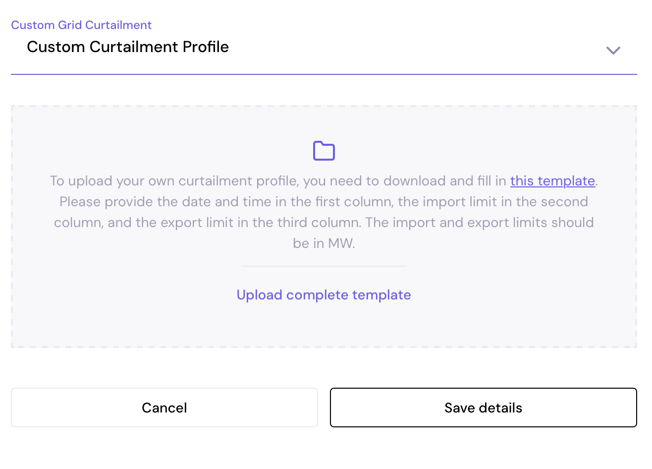
To create a curtailment template for a renewable-linked FCA, for example implemented by SH-Netze and across E.ON DSOs in Germany, use the Custom Curtailment CSVs builder.
Ancillary service capacity is capped by combined and per-market limits
Under an FCA, the capacity a battery can commit to ancillary services may be restricted in two ways: by a cap on each market individually, and by a per-timestep cap on all ancillary markets combined.
Both cap types are entered as the share of rated power that is ineligible for ancillary services, not the share available. A connection agreement permitting 30% of the asset in aFRR is therefore entered as 70% ineligible. Entering 0% applies no restriction; entering 100% removes the asset from that market entirely.
Four fields on the Grid connection tab set the ancillary caps
| Field | What it caps |
|---|---|
| Combined ancillary services restriction | Total capacity held across all ancillary products in any single settlement period |
| FCR restriction | FCR capacity alone |
| aFRR positive restriction | aFRR positive capacity and energy activation |
| aFRR negative restriction | aFRR negative capacity and energy activation |
The combined cap is applied independently to the charging and discharging directions. Where both a combined cap and market-by-market caps are set, both are enforced simultaneously and the more binding of the two governs in each period. A combined cap of 70% of rated power unavailable, sitting on top of individual caps, means the model can stack individual ancillary markets only up to that 30% ceiling.
These caps sit on top of the market rules that apply to every asset, and cannot be used to relax them. FCR remains derated to 80% of rated power, the 150 MW per-asset FCR cap still binds, and the state-of-charge energy reservoir requirements for ancillary delivery still apply.
- Reduced capacity: export constraints leave less of the battery available for FCR and aFRR.
- Applied in dispatch: ancillary provision is held within the FCA limits in every period.
- Revenue impact: comparing a constrained forecast with an unconstrained one quantifies the cost of the restriction.
A 100 MW asset with 70% ineligible on both caps holds at most 30 MW of aFRR positive
A 100 MW asset has the aFRR positive restriction entered as 70% ineligible and the Combined ancillary services restriction entered as 70% ineligible. It can hold at most 30 MW of aFRR positive. If it holds that 30 MW, the combined cap is already fully used, so no FCR can be added on top in that period. The remaining 70 MW stays available for wholesale energy dispatch, subject to the grid constraints.
Related Pages
- Custom Curtailment CSVs – Build a renewables-linked curtailment profile for a forecast run
- Dispatch Model – How the model optimizes battery dispatch across German markets
- Revenue Stack – Overview of available revenue streams in Germany