Standalone Solar Model
The standalone solar model provides a clear view of your solar project’s revenue stack and performance metrics. It calculates wholesale revenues along with key KPIs such as specific yield, load factor, capture rate, and losses from negative pricing or clipping.
It uses the same assumptions as our co-located Solar + Storage model for consistent results, supports flexible inputs (PVsyst files or site parameters), captures cannibalisation effects, and reflects negative-price behaviour to deliver realistic long-term revenue forecasts.
Note: For region-specific revenue mechanisms (e.g., CfD contracts, renewable certificates), see the regional documentation pages.
Solar Representation
Solar assets are represented in the model with the following key parameters:
- Nameplate Capacity (MW): Maximum power rating of the solar plant
- Coupling Type: AC or DC coupling, affecting efficiency losses
- Tracking Type: Fixed or Single-Axis Tracking (SAT)
- Positioning Parameters: Surface tilt and azimuth angles
- Loss Parameters: Shading, soiling, mismatch, wire, age, and availability losses
- Operational Configuration: Parameters controlling market participation and revenue mechanisms
Generation Modeling
The solar generation profile is modeled using either:
- Custom Profiles: User-provided generation profiles
- PVLib-Generated Profiles: Profiles generated using solar irradiance data and PV system specifications
The model accounts for two key components of solar generation:
Total Generation = Unclipped Generation + Clipped Generation
Where:
Unclipped Generationis the theoretical maximum generation based on available irradianceClipped Generationis generation lost due to inverter capacity limitations
Capturing Cannibalisation
As solar penetration increases in any market, wholesale prices tend to be lower when the sun is shining. This effect—known as cannibalisation—reduces the capture price for solar generators relative to the baseload price.
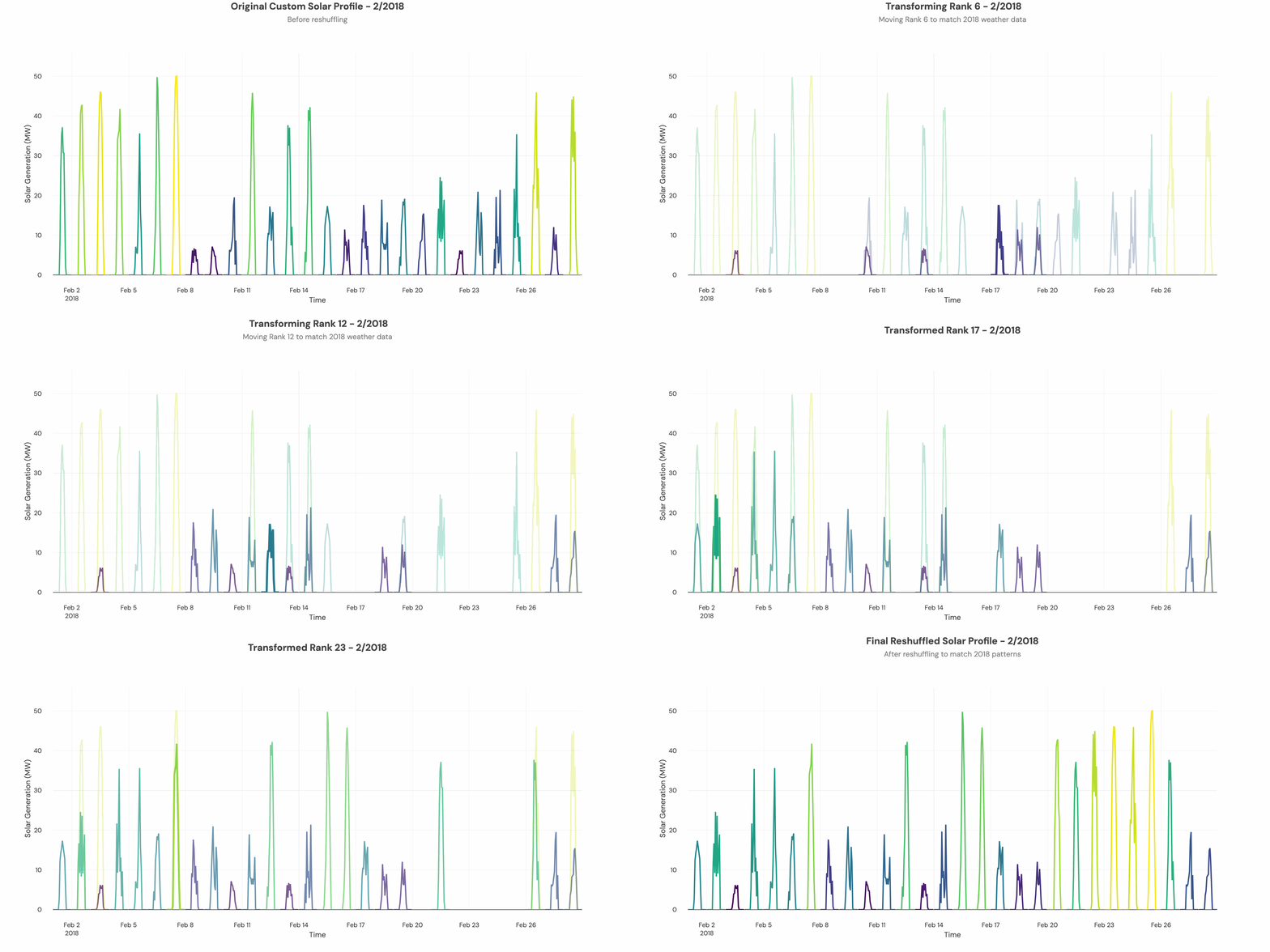
To capture cannibalisation accurately, it’s importnat that the solar generation profile is aligned with the weather year used in our Fundamentals Model.
To ensure this, we shuffle the custom solar profile within each month to ensure it better aligns with the 2018 weather year used in the Fundamentals Model.
For each month, we:
- Generate a reference solar profile for 2018 at the site.
- Rank the days in the 2018 profile by total solar generation.
- Rank the days in the input solar profile (whether custom or PVLib-generated) by total solar generation.
- Reorder the days in the input profile to match the 2018 ranking.
This process ensures that solar output and power prices are based on consistent weather conditions, avoiding overestimation of capture rates and revenues.

Physical Constraints
The solar model accounts for several physical constraints:
1. Inverter Clipping
When DC power from the panels exceeds the inverter capacity, excess generation is clipped:
Clipped Generation(t) = max(0, Unclipped Generation(t) - Inverter Capacity)
2. Efficiency Losses
AC-coupled solar systems experience additional efficiency losses:
Effective Generation(t) = Generation(t) × Efficiency Factor
Where Efficiency Factor is typically 0.975 (2.5% loss) for AC-coupled systems.
3. Grid Export Limits
Solar export is constrained by grid connection capacity:
Solar Export(t) ≤ Grid Export Limit
Integration with Battery Systems
When solar is co-located with battery storage, the model optimizes the allocation of solar generation:
1. Energy Balance
Solar Generation(t) = Grid Export(t) + Battery Charging(t) + Curtailment(t)
2. Battery Charging from Solar
Solar generation can be used to charge co-located batteries:
Battery Charging from Solar(t) ≤ Solar Generation(t)
Battery Charging from Solar(t) ≤ Battery Charging Capacity
3. Efficiency Considerations
When charging batteries from solar, the model accounts for efficiency losses:
Battery State of Charge Increase(t) = Battery Charging from Solar(t) × AC Efficiency × Battery Charging Efficiency
Revenue Calculations
The model calculates solar revenue across different mechanisms:
Merchant Revenue
Revenue from selling solar generation directly to energy markets:
Merchant Revenue(t) = Energy Price(t) × Solar Export(t)
If the solar asset is not exposed to negative prices:
Merchant Revenue(t) = max(0, Energy Price(t)) × Solar Export(t)
Region-Specific Revenue Streams
Additional revenue streams (contracts, certificates) vary by market. See regional documentation:
- GB Solar Forecast: CfD contracts, REGO certificates
Capture Price and Cannibalization
The model calculates key metrics to assess solar value:
1. Capture Price
The generation-weighted average price received for solar output:
Capture Price = ∑(Energy Price(t) × Solar Generation(t)) / ∑(Solar Generation(t))
2. Capture Rate
The ratio of capture price to time-weighted average market price:
Capture Rate = Capture Price / Average Market Price
A capture rate below 100% indicates that solar generation is correlated with lower-price periods.
3. Profile Delta
The difference between capture price and average market price:
Profile Delta = Capture Price - Average Market Price
A negative profile delta indicates cannibalization, where solar generation tends to coincide with lower market prices. This effect increases as solar penetration grows.
Model Outputs
The standalone solar model provides the following key outputs:
- Revenue Projections: Detailed revenue forecasts by revenue stream
- Generation Metrics:
- Total generation (MWh)
- Specific yield (kWh/kWp)
- Capacity factor / load factor (%)
- Market Value Metrics:
- Capture price (currency/MWh)
- Capture rate (%)
- Profile delta (currency/MWh)
- Loss Analysis:
- Clipping losses (MWh and revenue impact)
- Revenue lost during negative price periods
Regional Documentation
For market-specific revenue mechanisms and contract structures:
- GB Solar Forecast: CfD contracts, negative pricing rules, REGO certificates